I recently read the book “Following the Trend” by Andreas Clenow. It gives explicit details about how to construct a trend following trading strategy on futures using simple rules, and explores in some depth the performance over a wide variety of asset classes. As a means to learn more about algorithmic trading I thought it would be an interesting exercise to try to reproduce some of the results.
In this post I’ll just give a summary of what I’ve tried to do and give some examples of the end results. I’ll dig a bit deeper into the mechanics and some points of interest at a later date.
The R code is on GitHub here.
While the book covers a range of concerns you would need to consider when running a trend following trading strategy, such as sizing and asset mix, initially I’m just going to concentrate on coding up the trend following algorithm itself.
Time-series Data
Before thinking of running a back-test you obviously need the time-series data. The Quandl site has a large set of future time-series and it is very easy indeed to load them into R. However, by their very nature future time-series have an expiry date, and to get a full series you need to stitch these together. When it comes to actually executing a strategy you would normally aim to enter into the trade by buying/shorting the most liquid future in the series at that point. As you continue to hold the position you would then want to roll on the the next future in the sequence as that becomes more liquid. At the point of rolling there may be a basis spread, and you need to account for this when constructing the full series.
There are series available where this has been done for you, but I wanted to be faithful to the description of the algorithm in the book so I implemented it myself. There are numerous candidate rules for deciding when to roll, but the one used in my code and the book is to switch when the open interest (the total open positions) in the later future exceeds the open interest of the current future.
The Trend Algorithm
The algorithm makes use of a trend-filter that determines whether the overall direction of the asset price is either up or down. This is done by simply taking two moving averages of the price, one on a short span of say 50 days, and the other on a long span of say 100 days. If the shorter average is above the longer one then the price is in an upward trend, and vice-versa.
It also makes use of the Average True Range (ATR), which acts as a very simple measure of the series volatility. The true range is defined as the difference between the high and low for the day, taking into account the previous day’s close. The ATR is then the average over a given span of say 50 days.
The algorithm can then be summarised as:
- Long trades can only be entered if the trend filter indicates the overall trend is up, and inversely for short trades.
- If the criteria above is met, we enter a long trade if the closing price is the highest in the last 50 days; and conversely the lowest close for short trades.
- A long position is closed out if the closing price falls 3 ATR units from the highest point reached since entering the trade, with the equivalent applying to short positions.
Running the Code
Once the code is loaded a simulation can be run as in the example below.
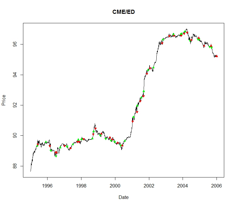
# Load CME euro-dollar between 1995 and 2005
ed_series = create_future_time_series(1995, 2005, 'CME', 'ED')

# Run a back-test on this data using the default parameters
ed_trades = run_simulation(ed_series$full_series, simulation_parameters())

# Print out trades and total pnl
ed_trades
sum(ed_trades$pnl)

# Plot the results
plot_trades(ed_series$full, ed_trades, title = "CME/ED")
A Sample Result
Running the euro-dollar example given above gives the output below.
> ed_trades
   position    date_in settle_in   date_out settle_out    pnl
1         1 1995-05-24    89.333 1995-06-07     89.433  0.020
2         1 1995-11-30    89.583 1996-02-20     89.323 -0.200
3        -1 1996-03-15    89.023 1996-06-27     88.893  0.110
4        -1 1996-07-05    88.653 1996-07-16     88.893 -0.230
5         1 1996-10-01    89.223 1997-01-02     89.333  0.070
6        -1 1997-02-27    89.283 1997-05-09     89.178  0.110
7         1 1997-07-02    89.428 1997-10-10     89.593  0.190
8         1 1997-10-27    89.728 1997-11-14     89.593 -0.240
9         1 1998-01-06    89.763 1998-02-19     89.778  0.020
10        1 1998-08-27    89.810 1998-09-15     90.088  0.222
11        1 1998-09-23    90.273 1998-11-02     90.473  0.225
12       -1 1999-02-12    90.033 1999-03-09     90.123 -0.070
13       -1 1999-06-11    89.803 1999-09-08     89.875 -0.057
14       -1 1999-10-05    89.680 1999-10-29     89.755 -0.050
15       -1 1999-12-20    89.592 2000-02-24     89.519  0.085
16       -1 2000-04-27    89.364 2000-06-02     89.354  0.000
17        1 2000-07-27    89.654 2001-01-12     90.939  1.319
18        1 2001-01-30    91.229 2001-04-16     91.554  0.370
19        1 2001-04-20    91.974 2001-06-28     92.279  0.255
20        1 2001-07-18    92.504 2001-09-04     92.609  0.165
21        1 2001-09-07    92.919 2001-11-16     94.069  1.142
22        1 2001-12-10    94.316 2002-01-24     94.434  0.038
23        1 2002-04-05    94.474 2002-10-11     96.086  1.495
24        1 2002-10-29    96.311 2003-03-13     96.548  0.255
25        1 2003-06-10    96.668 2003-06-25     96.573 -0.140
26        1 2003-11-14    96.658 2003-11-28     96.588 -0.120
27        1 2003-12-05    96.693 2004-01-29     96.708  0.030
28        1 2004-02-11    96.838 2004-04-02     96.788 -0.060
29       -1 2004-06-04    96.253 2004-06-30     96.303 -0.050
30       -1 2004-11-19    96.350 2004-12-08     96.425 -0.115
31       -1 2004-12-16    96.315 2005-04-06     95.910  0.380
32       -1 2005-08-01    95.845 2005-08-31     95.900 -0.057
33       -1 2005-09-12    95.790 2005-12-30     95.225  0.585

> sum(ed_trades$pnl)
[1] 5.697
So we can see we made just over 30 trades during the period and made a profit of 5.7 units. A quick count would show 20 winning trades and 12 losing ones.
However there are almost too many provisos to list here. In particular the algorithm as it stands assumes that a position can be entered or closed using the opening price the day after the signal. This doesn’t take into account the bid-ask spread or the slippage on the price. Nor are transaction fees factored in. However it does give a basic illustration of the effectiveness of trend detection using a very simple formula.
The plot looks as below. A green triangle is a trade entry, a red triangle an exit. A triangle pointing up is a buy/cover, pointing down is short/close. Although the presentation could do with some work you should be able to distinguish some of the key characteristics of this type of algorithmic strategy, namely that you can end up making quite a lot of small loses in a relatively flat market, but you can make relatively bigger gains when strong trends do emerge.