
In a previous post I described my attempts to replicate the trend-following algorithm from the book Following the Trend by Andreas Clenow. This post gives an update on my somewhat chequered progress since then.
Introduction
As a quick re-cap, trend-following is a trading strategy which is very much what it sounds like. You aim to detect that a trend is developing in a market and then trade as if that trend is going to continue. When it looks like the trend is over you close the trade. The book Following the Trend gives a very simple algorithm to do this.
As an example of it working well, here’s a chart of Palladium future prices in 2008, together with indications of where the algorithm decides to buy and to sell.
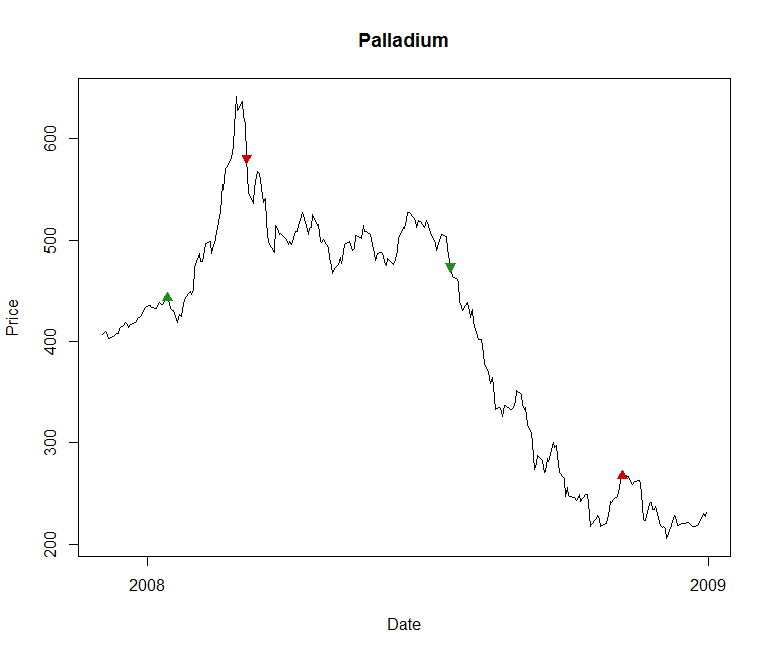
The upward green arrow in early 2008 indicates where it decides to buy into the rising market. A few weeks later the downward red arrow indicates where it has decided the trend has ended so it closes out the trade at a profit. Later in the year it picks up on a falling price trend, and the downward green arrow shows where it enters a short position. About three months later it picks up a signal that the trend has ended and so exits. This illustrates a couple of the benefits of trend-following as a strategy. First, it can profit from both a rising and falling market. Second, it can act as a good hedge against the equity markets that suffered significant falls across 2008.
To illustrate that it isn’t all plain sailing though, here’s an example of how it can fail. The graph below shows progress of the S&P throughout 1993.
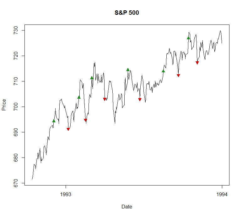
There’s a clear rising trend throughout the year, but the algorithm repeatedly enters long trades, as shown by the upward green arrows, only to exit them quite rapidly at a loss when it looks like the trend is over.
Project aims re-visited
My aim was to reproduce the return figures presented in the book, and in doing so gain some insight into algorithmic trading and to become more familiar with the R language. I’m afraid I’ve not really reproduced the results. For reasons I’ll go over I scaled back this target, instead settling for a sufficient implementation to gauge the strategy’s effectiveness or otherwise. Additionally, while the returns from my back-testing bare strong similarities to those in the book, there are also significant differences, overall being rather poorer.
However in doing the development and looking into reasons for the divergence I think I have learned quite a bit. My capabilities in R have advanced, though as I consider later this might not have been the right context in which to do it.
In this post I’ll give a summary where I’ve got to and discuss some drawbacks with the approach I took. I won’t analyse trend following performance too much, the book does that far better than I can, but I will pick out a few results which I think are illustrative.
Implementation summary
The code is here on GitHub.
At the point I first posted on this project I had a basic trend detection working. I was able to roll together the futures to create a full time-series, and run the basic algorithm to detect when to enter and leave a position. To build on that I’ve had to do the following:
- Make improvements to the rolling process, including some level of data-cleaning.
- Collect together static data on all the futures, including Quandl identifiers, point values and tick sizes. I also had to work out where there were gaps in the data, I only wanted to run backtests across continuous series.
- Add support for contracts that are quoted in different currencies, which involved loading the spot FX rates from Quandl.
- Add position sizing.
- Calculate the various costs to a trade.
- Introduce methods for loading, testing and reporting on multiple series at once.
Running the code
Running a test is a three step process: first you load up the futures time-series; then you run the test; finally you analyse the results.
The series are loaded this code.
full_series_set = load_all_future_series()
This loads up series for the 40 or so assets I was considering. For each it stitches the individual futures series together into a continuous whole. With futures expiring every three months or more, and data going back as much as 30 years, this means loading up in the order of 5000 individual time series. They are all sourced from Quandl, but I cache them locally.
Next we run the simulation. Tuning parameters can be set but there are defaults configured that match those given in Following the Trend. This step takes several minutes, which in truth is longer than you’d want if you were investigating the effect of changing different parameters.
sim_results = run_simulations(full_series_set)
Having run the simulation you can now investigate the results. There are all sorts of ways to splice and dice them to see how performance varies over time and by instrument.
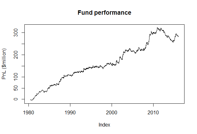
Here’s how to generate a nice plot that makes it look like the fund has done rather well.
cum_pnl <- combined_cumulative_pnl(sim_results)
plot(cum_pnl$cum_pnl/1000000, main="Fund performance", ylab = "PnL ($million)")
Here are the returns each year for which I have data, together with the compounded returns you could make if you were an investor and the fund employed the 2 and 20 model.
compounded_returns(sim_results, 1980, 2015, fixed = 0.02, perf = 0.2)
   year return compounded
1  1980  -2.07  0.9593278
2  1981  65.81  1.4452356
3  1982  29.77  1.7605852
4  1983   3.80  1.7788449
5  1984  34.50  2.2342338
6  1985  25.60  2.6471244
7  1986  13.11  2.8718665
8  1987  56.49  4.1122351
9  1988  21.72  4.7445700
10 1989   4.54  4.8219629
11 1990  23.78  5.6429633
12 1991   0.26  5.5419688
13 1992   6.77  5.7310966
14 1993  24.01  6.7172179
15 1994   7.33  6.9767663
16 1995   7.79  7.2717464
17 1996  -5.44  6.7308612
18 1997  -6.59  6.1523749
19 1998  32.49  7.6284059
20 1999  -8.53  6.8254129
21 2000   3.12  6.8594545
22 2001  46.33  9.2648429
23 2002  25.31 10.9556761
24 2003   9.43 11.5634457
25 2004  -1.94 11.1081567
26 2005   0.76 10.9537310
27 2006   1.93 10.9039788
28 2007  12.34 11.7622525
29 2008  60.51 17.2205622
30 2009  26.55 20.5336905
31 2010  25.19 24.2615806
32 2011 -11.21 21.0563015
33 2012 -31.60 13.9809975
34 2013 -20.96 10.7711249
35 2014  -9.89  9.4907652
36 2015  29.12 11.5117224
It should be pointed out the attribution of returns to a year is simplified a bit. What you would want to do is mark-to-market any positions you have at the start of the year and start from there, and do similarly as you end the year for any trades you have on at that point. Instead I’ve assigned PnL to the year in which the trade exits. So if a trade runs for several months, exiting early January, the PnL will be attributed to the year that has just started, even though all the profit came from the year before.
Leaving this aside, the take-away results are:
- There are big variations in performance across time.
- It did well when equities were doing badly, see 2001/2 and 2008.
- It took an almighty hammering between 2011 and 2014.
- The compounded returns I saw failed to match those from Following the Trend. The book saw a 40 fold increase on investment between 1990 and 2011, assuming a 1.5% and 15% charging structure. Changing the dates and the parameters to match this I only saw a gain of about 6 fold. I’m not sure of the reasons but I’ll speculate below.
This shows the return for each sector across the time-span used by the book.
pnl_summary_by_sector(sim_results, 1990, 2011)
I’ll explain the meaning of the numbers further down, but from the return figures you should be able to see that that rates, currencies and non-agricultural commodities did OK, while equities wasn’t so good.
                return      pnl   equity
Agricultural  7.429447 29420612 18000000
Commodities  17.329207 62038562 16272727
Currencies   19.036506 49875646 11909091
Equity        5.172984 11794404 10363636
Rates        17.581117 51688485 13363636
Finally, here’s how to see performance across individual future series from 2001 to 2010, the period for which I have the most data.
tt <- trade_list_summary(sim_results, 2001, 2010)[,c('annual_return', 'actual_pnl', 'theo_pnl', 'slippage', 'spread_cost', 'fees', 'duration')]
tt[order(tt$annual_return),]
This shows the actual pnl, plus a theoretical pnl. The difference between them is the various costs: transaction fees, bid-ask spread and slippage. A negative slippage is possible, meaning you trade at a better price than the one that generated the signal. The duration is the number of years for which the simulation ran, there’s some missing data.
               annual_return actual_pnl theo_pnl slippage spread_cost    fees duration
Lean hogs             -29.30   -5859362 -1886548  2480734      497360  994720       10
Oats                  -28.51   -5701982  -485962  2259625     1137075 1819320       10
Long gilt             -19.47   -3893157 -2073751   982181      386065  451160       10
Corn                  -17.70   -3539285     7200  1092800      943725 1509960       10
Short sterling        -14.73   -2945685 14021075   845061     8395859 7725840       10
Lumber                -12.88   -2575787  1909798  3295743      422202  767640       10
Nikkei 225             -5.08   -1016894 -1414707 -1479941      572568  509560       10
Silver                 -1.41    -282925  1546640   553545      708900  567120       10
CrudeOil               -0.68    -135360    13930  -550670      233320  466640       10
EuroSwiss              -0.16     -32192 12700871  3266829     4712355 4753880       10
Rough rice              0.25      49690  5065330  2563080      817520 1635040       10
GBP/USD                 2.37     473694  1708056   510650      172312  551400       10
Wheat                   3.67     733712  2830475   709988      533375  853400       10
CAD/USD                 4.25     850850  1105450 -1008040      420880  841760       10
Live cattle             4.32     863136  3766076  1037960      621660 1243320       10
Heating oil             5.74    1147246  1004060  -613053       81547  388320       10
S&P 500                 9.32    1863815  2015650  -639020      304175  486680       10
FTSE 100               11.14    2227331  2802202    71765      151707  351400       10
Soybeans               13.68    2736495  4865925   730825      537925  860680       10
Bund                   13.86    2772989  4047096   -20251      482318  812040       10
Natural gas            14.60    2919190  2342600  -961190      128200  256400       10
NZD/USD                16.91    2367170  3989420   963510      219580  439160        7
JPY/USD                21.39    4277710  6029688  1144238      144700  463040       10
Gold                   25.51    5102410  6082470   113600      288820  577640       10
Gasoil                 27.92    2233525  2898050   364825      166500  133200        4
US 10-year             29.55    5910612  6779940  -451576      579344  741560       10
Schatz                 29.71    5942143 11324087  1550353      888071 2943520       10
Hang Seng              29.96    5992121  4118045 -2256372       92976  289320       10
Nasdaq 100             31.24    6248426  6041591  -963935      151420  605680       10
Platinum               32.96    6591490  9050755  1621715      167510  670040       10
CAC Index              35.39    7077107  8073518   341403      154609  500400       10
EUR/USD                35.64    7127668  7436050  -204337      197200  315520       10
DAX                    37.00    7400111  8156845   489899      113835  153000       10
CHF/USD                45.40    9080542  9347937  -491675      291950  467120       10
AUD/USD                55.70   11139530 10919480 -1178910      319620  639240       10
Euribor                64.63   12925138 21142139  1647889     2771431 3797680       10
US 2-year              66.66    5332506  5911267   -93483      294844  377400        4
Copper                 72.61   14522680 15766737  -220263      563200  901120       10
Cotton                 85.73   17145815 19528115  1779100      120640  482560       10
Palladium              89.41   17881860 20364540  2006230       95290  381160       10
EuroDollar             97.10   19420236 27876435  1773809     2570150 4112240       10
I’ll later describe the assumptions behind these figures. However the main observation to make is that there is a huge variation in performance, from near a 100% annual return from EuroDollar, to almost 30% negative returns from lean hogs. One of the keys to performance in trend following is the need for diversification, and I think this illustrates pretty well why this is. If you pick only a handful of series you might be lucky and get the good ones, but you might not.
Just in case you look at these figures and think well “why not just trade the EuroDollar?”, let me tell you how it performed from 2011 to 2015. It averaged -86%. In fact in half the time period above it pretty much lost half the 2001-2010 gains.
Position sizing
I should describe what the various numbers mean in the context of my simulation, even though the details might not be of all that much general interest. First I need to introduce position sizing.
Position sizing in an algorithm is important, it controls the risk and hence how much can be made or lost. The formula presented in Following the Trend is simple, the number of contracts to be bought or sold is given by:
(Equity * Risk factor) / (ATR * Point value)
The equity is the amount invested in the fund. The risk factor is the variable that can be controlled to ramp the position sizing up and down. The ATR is the average true range, a volatility measure that indicates how much price movement might be expected in a single day, while the point value is the value of a point movement in a single contract. The denominator represents how much a single day’s movement might cost for one contract, so what we’re saying is we want to buy enough contracts that an average day’s movement might have a certain percentage effect on the fund value, and that percentage is the risk factor. It is set to 0.2% for each of the 50 contracts in the book.
Implementing this is straightforward enough, especially since the ATR was already being calculated, it is used in determining when to exit a trade. However the equity value appeared to present one problem, and I missed the fact that it also presented another.
Equity, pnl and return
The basic algorithm assumes an equal weighting of the nominal $100m fund equity across the 50 instruments under consideration. Of these 50 I only had time-series data across the full date range for about half and was completely missing 9. (I should point out that I think it’s pretty remarkable that Quandl makes as much as this available for free, and it might be that more is available if you’re prepared to pay for their premium sets.) Running with half the number of series, but keeping the equity the same, would have effectively halved the risk factor.
So what I decided to do was to treat each instrument as having $2m of equity, one fiftieth of the fund, but a risk factor of 10%, or 50 times the original. To be honest this makes the results I provide a little misleading. I’m saying that each instrument is being treated as a mini-fund with $2m worth of equity. But I’m in not restricting the loses if they exceed that, which they often do. So what the numbers mean are this:
- Equity – There is a nominal $2m equity provided for each traded future.
- Risk factor – The risk factor is set so that the contract sizing will match that in the book, i.e. as if there were 50 futures being traded with a starting equity of $100m and a risk factor of 0.2% each.
- PnL – This is the (non-compounded) gain made across the test period. Perhaps rather illogically, loses can exceed the equity. This is allowed because the equity is pooled across all instruments, and so (hopefully) aggregate losses won’t exceed total equity.
- Return – The average return across the time period, the return being (PnL / equity). If there is only limited data for an instrument across the period, only those years for which data is used are considered and the equity is scaled accordingly. When instruments are combined for analysis, for example when looking at results by sector, in effect these returns are averaged, not added together.
The overall effect of all this is that it allows the risk factor to match what I’m comparing against, and it provides a means of comparing performance across futures with different amounts of data available in a fair manner.
Compounding the error
I’ve learned a valuable lesson in how not to implement a backtest.
My implementation treated each future series independently, which seemed like a reasonable thing to do as trade algorithm works on a single instrument in isolation. So I developed my code to run through each series under consideration before then combining the results. This works fine for determining the trend performance on a per-contract basis. However it doesn’t allow for the calculation of overall fund performance. The difference, in a word: compounding.
When calculating overall fund performance the series aren’t in fact independent. Say you have a fund with just two future instruments in the portfolio. If after one year one has exactly broken even, but the other has doubled its money, then the equity in the fund will have gone up 50%. This equity will now be available to both instruments, scaling up the position sizes as per the equation given above. It’s this compounding effect that can give an exponential increase in fund size if it is successful, and unfortunately my current implementation has no means to replicate it directly.
I’ve made an attempt to examine compound returns, as per one of the example illustrations of the code above. However this is only an approximation. It only considers end-of-year returns, when compounding should be continuous based on when a trade is closed out and the profit taken. Furthermore, these annual returns themselves aren’t all that accurate due to the lack of mark-to-market at year-end that was mentioned above.
Trading costs
In one of the examples I gave above there is a theoretical PnL figure. This is the PnL you would achieve if you were able to trade at the settlement price used to generate the trading signals. The simulation considers three costs that mean the actual pnl differs from this: slippage, bid-ask cost and broker fees.
The fees were the easiest to calculate. As per the assumptions stated in Following the Trend, a $20 per contract traded fee was assigned. This applies not only to the trades to enter and exit a position, but also any time the position needs to be rolled from one contract to the next.
Slippage is due to not being able to trade at the settlement price. I just made the assumption that you could trade at the opening price on the day after the signal had been generated. This means it could actually act in your favour and not be a cost at all. If you decide to buy, and the price then drops the next morning, you still buy but get it at a better price. On balance though it will be a cost, since if you are buying only in a rising market then the open is likely to be higher than the previous settle.
Any market is going to have a bid-ask spread. The time-series data I was working off didn’t give me any guide to what it was likely to be so I made an enormous sweeping assumption. I just assumed the bid-ask spread would always be the minimum tick-size either side of the mid. So each time I traded a contract, including when rolling in and out, I would pay the minimum tick-size times the point value (i.e the minimum price movement). My guess is that this might not be ridiculous for highly liquid futures, however it could be miles out for others.
I’m not a market participant, I don’t trade futures, and I don’t know if the above represent realistic assumptions. I plan to talk to a couple of practitioners to get their view.
Explaining the performance
As mentioned above, the performance I saw from the algorithm didn’t match that given by Following the Trend. Over the period covered by the book, 1990 to 2011, my simulation yielded an increase in investment of around 6 times, while the book managed about 40. I can’t tell exactly why this is but there are a few possibilities.
One obvious difference is that I didn’t attempt to replicate the effect of interest that you can get on excess cash. Because futures trading has relatively low cash demands, compared to trading underlyings such as equities, you can operate with a significant cash surplus. If you buy government bonds with this spare cash you can get a pretty-much risk free boost to your performance. This seems extraordinary. Investors can entrust you with capital on the basis that you’re going to generate returns for them using a systematic trading model, and all you do with a large amount of the cash is buy government bonds, something they could have done themselves without paying fixed and performance fees for the privilege. I learned from Following the Trend that this is exactly what happens, or at least what happened.
There are a few reasons I didn’t attempt to replicate this. It would require working out margin requirements across all the instruments, and making assumptions about how much liquid cash you would require in each currency you are trading with. Further, in today’s virtually interest free environment it doesn’t really apply, for instance Switzerland where I live currently has negative yields. It also might not be that interesting to model.
However by my calculations, even if you took away the effect of this free money from the returns in Follow the Trend it would have yielded a 24 times return on investment, still much better than my simulation.
The most obvious other source of differences is that I don’t have a full set of time series for all the futures used in the book. Of the 50 in the portfolio, I only had full data for about half of them. So although I adjusted to make sure the risk levels matched, there is a good chance with my less diversified portfolio I was missing out on some of the better performers. I suspect this was the primary source of differences, especially as my performance matched that in the book more closely for later years where I did have more complete data.
I could, of course, just have made some mistakes in implementation. I’m pretty sure the basic implementation is about correct. The book gives a sample set of positions that a portfolio would have on a certain date. My code gives a very close match to the positions and when they were entered.
However I have a far less good match for the position sizes. What this suggests to me is that there may be differences in the time-series data, in particular the daily high and low values. These are used in calculating the ATR, which in turn is used in position sizing and trade exit timing. It seems plausible that the settlement prices I used are pretty similar to the book’s. The settlement price is going to be far more trustworthy that any other data such as open, close or high since the settle price is used in official calculations. However the other prices can be noisy, missing or otherwise inaccurate. I’m not sure this is likely to be a big cause of performance differences, but it does mean that replicating exact results is harder.
A further difference could well come from the cost assumptions described above, not all the equivalent assumptions used in the book are explicitly stated.
Some thoughts on R
As mentioned above, one reason for the project was to improve my R programming skills. This seemed like a good idea at the time, but I still suffer from some of the frustrations I mentioned in the past.
If you know what you’re doing it can be very expressive. If you have some familiarity with the language and you know the structure of the data set you’re dealing with you can quickly delve into interesting data relationships interactively.
However despite being a useful analytic tool, I don’t think it was a great choice for a backtester, at least not in my amateur hands. Efficiency in R is achieved by avoiding loops, and particularly by not growing data-structures of an unknown size within loops. Unfortunately that’s exactly what I’m doing inside the backtest since the natural way to implement it is to step through time, maintaining state and growing structures that hold the trade information. I’m sure there are plenty of ways to improve what I’ve done, but I expect that implementing a more vectorised approach would make things less flexible and harder to debug.
The real power in R comes from the large set of statistical models that are readily available. For instance the only other time I used R in the past was to perform analysis on vector auto-regressive processes, such as applying the Augmented Dickey-Fuller and Granger Causality tests. However in this trend analysis I’m not using anything more sophisticated than a moving average.
I think if I were to start again I would look into using Python with the NumPy, SciPy and Matplotlib modules.
Conclusions
The primary aim of embarking on this project was to learn a bit about algorithmic trading. I’ve done that, especially some things not to do. In particular, if I were to implement a backtesting algorithm again I’d cater from the outset for two things I overlooked:
- Allow for valuing the state of the portfolio at an arbitrary point in time by marking any in-flight trades to market. My current implementation only allows for PnL to be calculated on completed trades.
- Run the backtest for all instruments under consideration in parallel. One example of their inter-dependence was given above, the accumulation of equity, but there could be others such as risk and cash management.
Other than that, this exercise has reinforced some lessons from the book. Trend following can be very profitable despite its simplicity, and diversification is a key element in achieving this. However it’s no golden bullet, under unfavourable market conditions it can also perform very badly.